Following up on our first post on the subject, Topic Modeling of Twitter Followers, we compare different unsupervised methods to further analyze the timelines of the followers of the @alexip account. We compare the results obtained through Latent Semantic Analysis and Latent Dirichlet Allocation and we segment Twitter timelines based on the inferred topics. We find the optimal number of clusters using silhouette scoring.
A word on LDA and LSA
We are in the context of latent topic modeling an unsupervised technique for topic discovery in large document collections. We try to analyze the topics underlying a given set of documents through a bag of word approach. Words are only considered according to their relative frequency and not according to their order within the document.
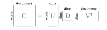
LSA is a vector-based dimension reduction technique that allows to project a large feature space unto any reduced number of dimensions. Used in the context of document analysis, words are considered features, their relative frequency (TF-IDF) are calculated and the matrix of document / word frequency is reduced through a classic Single Value Decomposition (SVD).
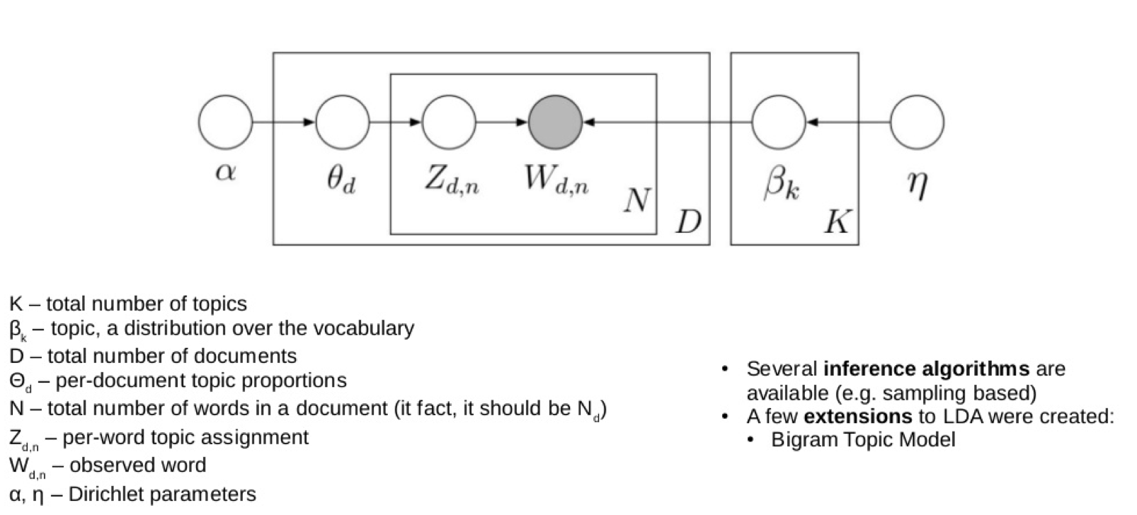
LDA is based on a bayesian probabilistic model where each topic has a discrete probability distribution of words and each document is composed of a mixture of topics. In LDA the topic distribution is assumed to have a Dirichlet prior which gives a smoother topic distribution per document.
See A Survey of Topic Modeling in Text Mining by Alghamdi and Alfalqi for a recent article on these and other (pLSA) topic modeling techniques.
Topic modeling and segmentation of twitter followers
LDA topic modeling is not the most reliable method to extract topics from twitter feeds that are composed of tweets, short texts which are by nature unstructured, full of invented words and in general very noisy.
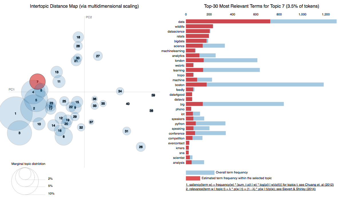
In a previous post, we used Latent Dirichlet Allocation to extract the topics of a given set of timelines. Although interesting in that the main topics were detected, these results could be improved upon. The most obvious problem is the ‘impurity’ of detected topics as most topics include words that obviously do not belong in the said topic. For instance, in our previous analysis, we had found topic #7 (see fig below) is about data science and machine learning, but the second most important word detected for that topic is the word: wildlife. (see also the last model in this notebook for a more interactive representation). It’s true Data science is a jungle of algorithms but so far no lion has been spotted (except maybe in Neural Network imagery).
In this post we would like to further develop the topic modeling analysis and the segmentation of the twitter followers of the @alexip account using the somewhat simpler Latent Semantic Analysis algorithm (LSA) algorithm. To give this algorithm all possible chances we will be more restrictive when it comes to building our corpus.
We
- build a better corpus of twitter timelines and focus on accounts that are active and not spamming,
- carry out dimension reduction with LSA in scikit-learn,
- segment the followers with K-Means clustering,
- and compare the results obtained with LSA and LDA.
The related python code is available here
- Extract follower timelines from Twitter
- Clean and Tokenize Timelines
- LSA and K-means
- Running LDA on previous corpus and dictionary
The raw and tokenized data is also available as a json file - 3Mb gz.
MongoDB database
Using a MongoDB database to store the data from twitter turned out to be extremely useful as our schema evolved from raw_text and user_id to include tokens, screen_names, metrics on the tweets, texts and tokens, and flags to select the right collection of documents in our different analysis. MongoDB is easy to install and quite simple to get started with (see this pymongo tutorial for instance)
Corpus of twitter timelines
The corpus is built around the aggregation of tweets into a document thus giving us a unique document per timeline. Since the first article was published a week ago, the @alexip account has gained about 50 more followers. For the most part, people interested in NLP and Machine Learning. Thus we updated the initial corpus by adding the new timelines.
As mentioned earlier, a twitter timeline is much more noisy than a more structured text such as a newspaper article. To improve upon our previous model we will further restrict the number documents on which our analysis is based.
- We only consider tweets that are less than 6 months old.
- We record the number of tweets per timeline and the length of the document to further filter out documents that have too little content. In fact we only kept 75% of the largest documents.
As usual a decent amount of time was spent cleaning up the documents.
- We removed non english timelines, first by filtering on the declared language of the Twitter account and secondly by using the langid language detection package. This way we remove timelines that are declared ‘en’ but contain tweets in other langages.
- We created a stopword list by aggregating words with one or two characters, NLTK stopwords for English and other languages (in case some non-English tweets leaked through) and a list of words that we found brought no meaning to topics during our successive iterations. Further ameliorations could probably be obtained by tagging words (nouns, adj., verbs, … ) and removing words of a certain type.
Twitter accounts can include a wide variety of users: robots, companies, real humans, news feeds, abandoned accounts, spam accounts, intensive retweeters, etc, … and specific accounts can end up having a disproportionate impact on the corpus. For instance a set of accounts tweeting about a very specific niche subject and tagging each tweet with the same hashtag would boost the influence of that word in the corpus.
After many runs of the LSA algorithm we decided to remove some accounts that displayed that type of timelines. The word bitcoin was preponderant in about 6 timelines and was heavily skewing our results. To detect such accounts, that displayed one dominant keyword, we used the TF-IDF matrix . In the end 7 accounts were removed from the set: ‘stickergiant’, ‘freemagazine’, ‘GigaBitcoin’, ‘B1TCOIN’, ‘1000btcpage’, ‘CoinUpdates’, ‘Cryptolina’.
We ended up with a corpus of 245 documents.
Performance of LSA dimension reduction and KMeans clustering
We tried many variants for the components (dimensions) of the LSA and the number of clusters of the KMeans. In order to assess the quality of our runs we used silhouette scoring which is a measure of the tightness of the different clusters. It is derived from calculating the distance of a given word with other words in the same cluster (a, low) and the distance with the words in the nearest cluster (b, high). Silhouette scoring is available in scikit-learn.
Hyperparameter optimization was carried out through a grid search on the number of dimensions [6, 12, 18, 24, 30] versus the number of cluster (2 to 60).
We found that for the lower dimensions, there was an optimal number of clusters maximizing the slhouette score. While for 30 dimensions, the curve reaches a maximum and then plateau. For higher dimensions we observed the same plateau. In all cases, there is no significant increase of silhouette score after a certain number of clusters. When the score curve shows a local maximum, this can be used to select the optimal number of clusters.
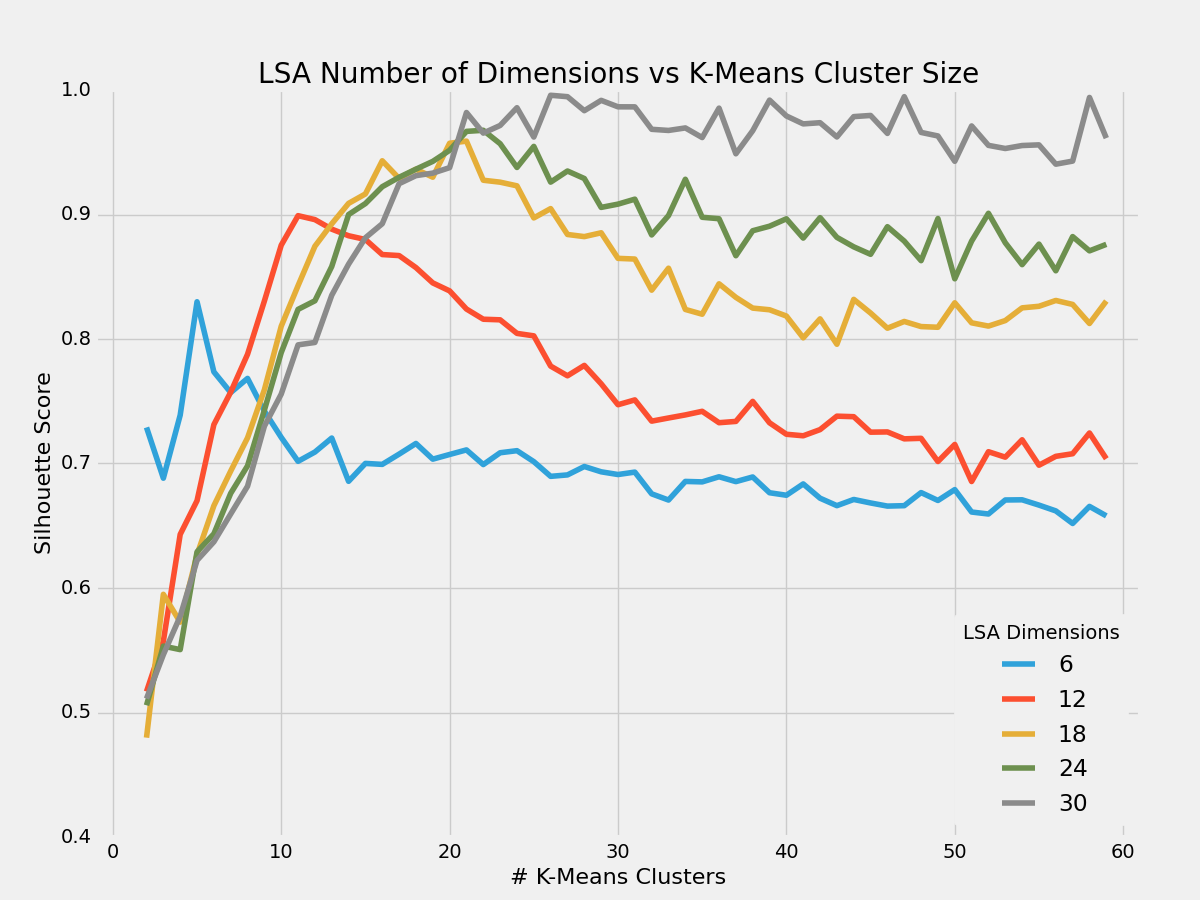
Note: Silhouette score drop as the dimension number increases. To compensate the silhouette score shown above is multiplied by the sqrt(n_dimension).
Silhouette scoring can also be used to visually assess the pertinence of the number of clusters. See a nice scikit based example
Visualization
Of course representing 40 dimensions on a 2 or 3 dimension plot is impossible. We thus revert to 2 dimensions for visualization purposes only. The LSA method result in the following topics composed of very similar words. Notice that data is the most prominent word in both topics. Notice also that Topic 2 has a global weight of ~3 times the weight of topic 1.
- Topic 0) weight: 0.13 0.183data 0.152time 0.120people 0.108learning 0.101think 0.100work
- Topic 1) weight: 0.35 0.529data 0.441datascience 0.375bigdata 0.234python 0.185learning 0.185machinelearning
Once in that 2 dimensions space, we can see in the figure below that most followers are tweeting on things very close to the first topic while minority is more spread out. The 2 topics do not discriminate well between the followers.
Comparing 2 vs 4 clusters
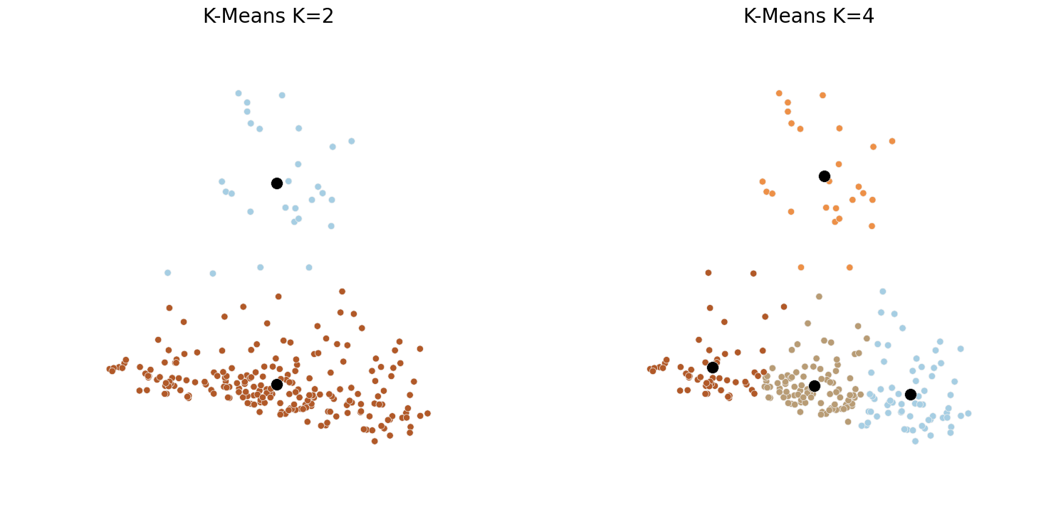
The respective silhouette scores for 2 and 4 clusters are 0.644 and 0.443 indicating a significant improvement for K=2. We can observe in the figure below that 2 is indeed the number of clusters that makes the most sense as predicted by the silhouette scoring above. Although we could segment the space into more clusters with good visual results, the global shape of the data clearly shows 2 blobs, with a major one (Topic 2) and a minor one (Topic 1).
Higher Dimensions
As we increase the number of dimensions for LSA, we do not observe a significant improvement in topic discrimination. On the contrary, LSA fails to detect any topic beyond the major ones and ends up with very mixed and similar topics.
For 5 topics: 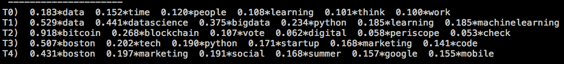
While for 15 topics: 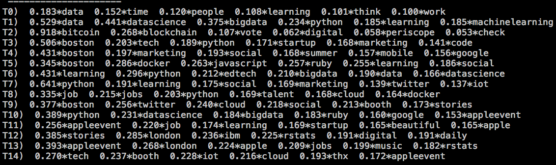
LSA appears to work better for a small number of dimensions. For 5 dimensions we have 4 well delimited major topics: Data Science (topics 1 and 2), Bitcoin (3), marketing & startups (4) and Web development (5)
For 15 topics, the distinction between topics is more blurry. Some words (stories, python, datascience) belong to 5 topics or more and some topics are very similar to each other:
LSA with even more topics (40, 100) also failed to detect topics that could were detected by LDA: Food, Music, Recruitment and Jobs, Martha’s Vineyard, JewishBoston, Fantasy Football, wildlife etc …
Comparison with LDA
We ran the LDA algorithm on our new updated corpus to compare with the LSA results.
The topic repartition is much better and much more discriminative than with LSA as shown by the ipython Notebook. Our optimal number of topics is 40. We trained the LDA algorithm (Gensim version) with 200 passes, alpha =0.001 and beta as the default value.
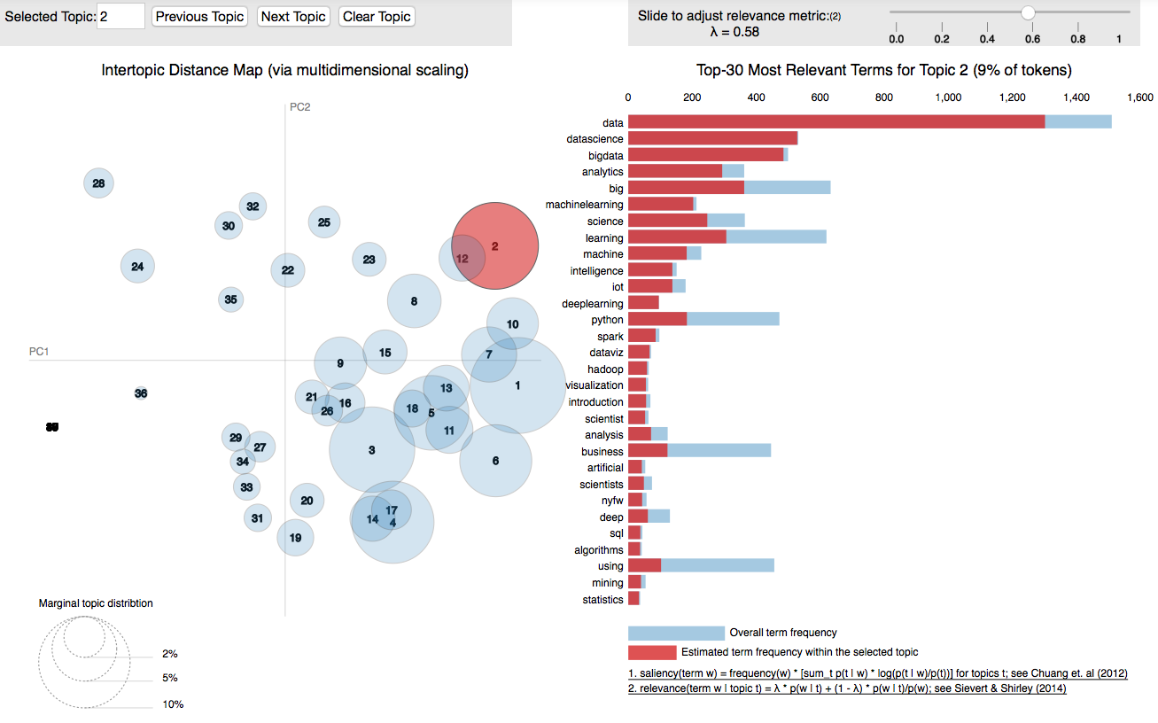
All the topics are visible in this notebook thanks to the amazing LDAvis package.
Some topic such as Data Science (T2) (see also Fig. below), Bitcoin (T7), Programming (T1) are very well defined, ; we see new topics emerging that were not detected by LSA: Conferences (T5), Fantasy Football (T4) or Martha’s Vineyard (T19), PMP and Project Management (T8), Fenway (T31), the list could go on….
Conclusion
As shown by the segmentation, it appears that the followers of the @alexip account are composed of a main techno-crowd tweeting on all things related to the Internet, software development, crypto currencies and Data Science and a much more diverse set of individuals mostly writing about one specific subject that is not related to anything software. This last group of people is very diverse in its center of interests.
Which means that the task that was asked of these topic modeling algorithms was to detect the finer subtile differences in a rather homogeneous large set of documents while at the same time still being able to find topics in a much smaller and far more heterogeneous set of documents. A difficult challenge.
In the end, combining segmentation through LSA and K-Means with topic modeling through LDA gave us a pretty accurate picture of the composition of the corpus. LSA was not able to detect the scattered topics but associated with K-Means for segmentation showed the overall structure of the corpus. LSA’s raison d’être is dimension reduction. LDA on the other end did a pretty decent job discerning the topics in the swarm of techno topics while also shining a light on the scattered topics. The 2 methods do complement each other.
One thing we mentioned earlier is that in this second part of the topic modeling of Twitter followers, we were more strict in building the corpus. This benefited LDA significantly. Comparing the topic definition and distribution in the first notebook and the second one, shows a much better topic repartition in the second one.
Further potential ways to improve the results may include using a variation of LDA for topics modeling such as seeded LDA to jumpstart the LDA algorithm or the Structural Topic Modeling package in R. Tagging the words by their nature to keep only nouns and verbs could also boost the quality of the corpus and lead to better results.
Structural Topic Models
[11/12/2015]
I have recently come across the Structural Topic Model R Package which among other things solves the main problem of finding the initial optimum number of topics. See the following article for an application of the STM model to the 2015 presidential debates: Dissecting the Presidential Debates with an NLP Scalpel